
Gradient Descent And Kernel Machines
Introduction
Domingos et. al demonstrate a relation between the similarity of training data samples and the inference point over the history of the changes of parameters for any model learned by gradient descent[1].
Assuming a model \(f(x; \omega)\), parametrized by weights \(\omega\) and taking input \(x\), they arrive at the following interesting result:
\[\lim_{\epsilon \rightarrow 0} y = y_0 - \int_{c(t)}\sum\limits_{i=1}^{m}L'(y_i^*, y_i) \vec{\nabla}_\omega f(\vec{x}; \vec{\omega}(t)) \cdot \vec{\nabla}_\omega f(\vec{x}_i; \vec{\omega}(t)) dt \tag{1}\]
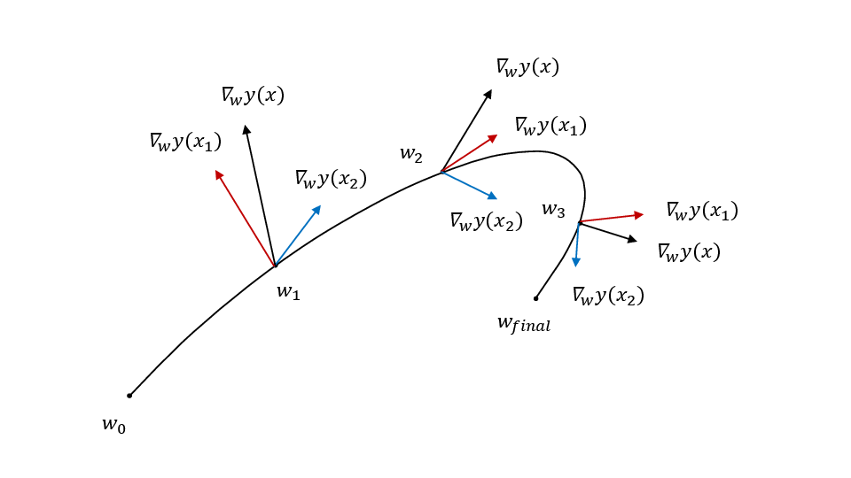
What this suggests is that no matter where our model starts (\(y_0\)), the movement towards the trained model can be approximated as a sum of terms weighted by the similarity between the gradient of the inference point \(\vec{x}\) and the training data point. This suggests that for a smooth enough parameter space, that the strongest contributing terms in the sum are the ones where the vector \(\vec{x}\) is closest. Intuitively, this is because some correlation of gradients for neighboring points can be assumed but no correlation (i.e. random) for other points.
The Open Question
The current scheme uses gradient flows [2] and requires that the learning rate \(\epsilon\) be very small. During training, it remains an open question whether this approximation holds. In particular, it assumes the system is not in a local minimum. Being in a local minimum would require jumping over a max (and reach a point where \(\epsilon=0\)).
They mention[1]:
This is standard in the analysis of gradient descent, and is also generally a good approximation in practice, since the learning rate has to be quite small in order to avoid divergence (e.g., \(\epsilon = 10^{-3}\)) [3]. Nevertheless, it remains an open question to what extent models learned by gradient descent can still be approximated by kernel machines outside of this regime.
Intuitively this makes a bit of sense. Practically, we observe this with basic LLMs where when giving a very simple prompt asking to solve a math specific question with the prefix “You are an MIT student” leads to a higher likelihood of a better answer than without.
This document aims to discuss what happens outside of this regime. How is this approximation affected? To what extent does it still hold?
Discrete Proof
Before discussing the limits, a discrete version of the original proof [1] must be derived. A key insight needed for this proof is the assumption that the model can be approximated by a hyperplane (i.e. can be Taylor expanded keeping up to first order derivative terms).
During gradient descent, weights are updated according to a rule: \[\vec{\omega}_{n+1} = \vec{\omega}_{n} - \alpha_{n+1} \vec{\nabla}L(\vec{\omega}_n)\]
where \(\alpha_{n+1}\) is the learning rate, \(\vec{\omega}_n\) the weights at timestep \(n\) and \(L\) the loss. Note that the loss is implicitly dependent upon the training samples \((x_i, y_i^*)\).
As in [1], the gradient of the total loss can be rewritten in terms of a sum over individual gradient losses with respect to the input:
\[\begin{aligned} \vec{\nabla}L(\vec{\omega}_n) & = & \sum \limits_j \frac{\partial L}{\partial \omega_j}(\vec{\omega}_n) \hat{\omega_j} \\ & = & \sum\limits_{j, m} \frac{\partial L}{\partial y_m} \frac{\partial y_m}{\partial \omega_j} (\vec{\omega}_n) \hat{\omega_j}\\ & = & \sum\limits_m \frac{\partial L}{\partial y_m} \vec{\nabla}_{\omega} f(\vec{x}_m; \vec{\omega}_n) \end{aligned}\]
summing over \(m\) training data points with \(y_m = f(\vec{x}_m; \vec{\omega}_n)\). Finally:
\[\vec{\omega}_{n+1} - \vec{\omega}_{n} = -\alpha_{n+1} \sum\limits_m \frac{\partial L}{\partial y_m} \vec{\nabla}_{\omega} f(\vec{x}_m; \vec{\omega}_n) \tag{2}\]
The change of the model at each timestep is: \[\Delta f = f(\vec{x}; \vec{\omega}_{n+1}) - f(\vec{x}; \vec{\omega}_n)\]
\(f\) can be rewritten as a Taylor series, centered at \(\vec{\omega}_n\): \[f(\vec{x}; \vec{\omega}_{n+1}) = f(\vec{x}; \vec{\omega}_n) + \vec{\nabla}_\omega f (\vec{\omega}_n) \cdot \left (\vec{\omega}_{n+1} - \vec{\omega}_n \right ) + O\(|\omega|^2)\]
The key step here is assuming that the function can be approximated by a hyperplane. This allows ignoring the <span class=\"math inline\">\(O\(|\omega|^2)\)</span> terms.
If this holds, the delta can be written as:
\[\begin{aligned} \Delta f & = & f(\vec{x}; \vec{\omega}_{n+1}) - f(\vec{x}; \vec{\omega}_n) \\ & = & f(\vec{x}; \vec{\omega}_{n}) - \vec{\nabla}_\omega f \cdot \left (\vec{\omega}_{n+1} - \vec{\omega}_n \right ) - f(\vec{x}; \vec{\omega}_n) \\ & = & \vec{\nabla}_\omega f \cdot \left (\vec{\omega}_{n+1} - \vec{\omega}_n \right ) \end{aligned}\]
Replacing \(\vec{\omega}_{n+1} - \vec{\omega}_n\) with Equation 2, we get:
\[\begin{aligned} \Delta f & = & - \alpha_{n+1} \vec{\nabla}_\omega f(\vec{x}) \cdot \sum\limits_m \frac{\partial L}{\partial y_m} \vec{\nabla}_{\omega} f(\vec{x}_m; \vec{\omega}_n)\\ & = & - \alpha_{n+1} \sum \limits_m \frac{\partial L}{\partial y_m} \vec{\nabla}_\omega f(\vec{x}; \vec{\omega}_n) \cdot \vec{\nabla}_{\omega} f(\vec{x}_m; \vec{\omega}_n) \end{aligned}\]
Finally, the final model will just be the sum of the \(\Delta\)s plus the initial model:
\[f(\vec{x}; \vec{\omega_N}) = f(\vec{x}; \vec{\omega_0}) + \sum \limits_{k=0}^{N-1} -\alpha_{k+1} \sum \limits_m \frac{\partial L}{\partial y_m} \vec{\nabla}_\omega f(\vec{x}; \vec{\omega}_k) \cdot \vec{\nabla}_{\omega} f(\vec{x}_m; \vec{\omega}_k)\]
yielding: \[\begin{array}{rcl} f(\vec{x}; \vec{\omega_N}) & = & f(\vec{x}; \vec{\omega_0}) + \\ & & \sum \limits_{k=0}^{N-1} -\alpha_{k+1} \sum \limits_m L'(y_i^*, y_i) \vec{\nabla}_\omega f(\vec{x}; \vec{\omega}_k) \cdot \vec{\nabla}_{\omega} f(\vec{x}_m; \vec{\omega}_k) \tag{3} \end{array}\]
which is the discrete version of Equation 1. Note that this is a similar result, except that the learning rate can be variable so long as the function can locally be approximated by a hyperplane.
Discussion
Not Quite Kernel Machine With Local Minima (But Still Approximate?)
Equation 3 demonstrates that it is sufficient to assume the method is locally approximated by a hyperplane at each time step.
It is evident that this breaks down when the assumption fails. When can this happen? This can happen where the slope of the approximate hyperplane is negligible and higher order terms must be kept. This could occur if the system is in a local minimum or saddle point. In one dimension, this is easy to visualize.
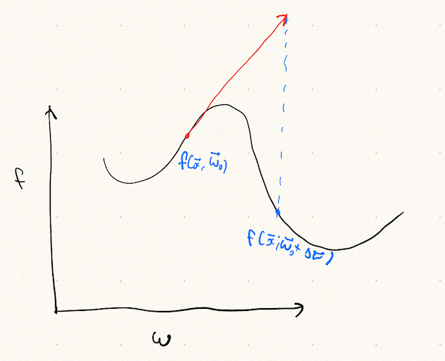
See Figure 2. Reaching the global minimum requires moving a \(\Delta \vec{\omega}\) where \(f\) cannot be approximated by the first order terms in \(\omega\). In this case, additional terms must be accounted for. Roughly, the Taylor approximation cannot be ignored. Grouping the complex timesteps into \(T_c\). This results in a sum like:
\[\begin{aligned} f(\vec{x}; \vec{\omega_N}) & = & f(\vec{x}; \vec{\omega_0}) + \nonumber \\ & & \sum \limits_{k=0}^{N-1} -\alpha_{k+1} \sum \limits_m L'(y_i^*, y_i) \vec{\nabla}_\omega f(\vec{x}; \vec{\omega}_k) \cdot \vec{\nabla}_{\omega} f(\vec{x}_m; \vec{\omega}_k) \nonumber \\ & & + \sum \limits\_{\omega\_k \in T\_c} + O\(|\omega\_{k+1} - \omega\_k|^2) \end{aligned}\]
Whether these terms contribute or not is an open question, and something that will have to be empirically determined. Roughly, it is likely related to the ratio of local minima encountered to total steps. Training usually involves some sort of regularization which attempts to smooth the space. This ratio is expected to be small, and likely there to be little contribution.
Kernel Machine When Initialized
Note that a simple solution to this problem would be to simply initialize parameters close to the global minimum. However, this weakens the kernel machines argument. Gradient descent is only a kernel machine if initialized near the solution.
Follow Up
Janko-dev’s notebook demonstrates this empirically. By tweaking the paths and ensuring the system is in a local minimum, it is possible to observe agreement or discrepancy, and how big the <span class=\"math inline\">\(O\(|\omega|^2)\)</span> terms are.
Citation
@misc{jlhermitte2025kernelmachine,
  title={Gradient Descent And Kernel Machines},
  author={Julien R. Lhermitte},
  year={2025},
  howpublished={\url{https://jrmlhermitte.github.io/2025/08/08/gradient-descent-and-kernel-machines.html}}
}